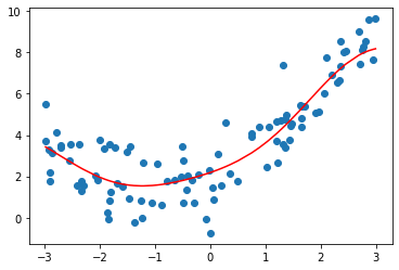
SVM（Support Vector Machine）

SVM tries to find a decision boundary (hyperplane) that is as wide as possible, keeping the data points from both classes as far from the boundary line as they can be.

I. Core Formulas and Mathematical Concepts of SVM (Basics)

1. Objective Function of Linear SVM (Optimization Problem)

We aim to find a hyperplane defined by the equation:

$$\mathbf{w} \cdot \mathbf{x} + b = 0$$

Where:

• $\mathbf{w}$: the normal vector (determines the orientation of the hyperplane)
• $b$: the bias term (determines the position of the hyperplane)
• $\mathbf{x}$: the input data point

Classification Decision Rule:

• If $\mathbf{w} \cdot \mathbf{x} + b \geq 0$, the sample is predicted as class +1; If $\mathbf{w} \cdot \mathbf{x} + b < 0$, the sample is predicted as class -1.

2. Objective Function for Maximizing the Margin

The core idea of SVM is to maximize the classification margin.

This margin is defined by the following formula:

$$\text{Margin} = \frac{2}{\|\mathbf{w}\|}$$

Therefore, our problem becomes an optimization problem:

$$\min_{\mathbf{w}, b} \frac{1}{2} \|\mathbf{w}\|^2 \quad \\ \text{s.t. } y_i(\mathbf{w} \cdot \mathbf{x}_i + b) \geq 1$$

• This is a typical constrained convex optimization problem and the goal is to minimize $\|\mathbf{w}\|$, which in turn maximizes the margin.

3. Introducing Slack Variables (Soft Margin) — Allowing Misclassifications

In real-world datasets, perfect linear separability is often not possible. To handle this, we introduce slack variables $\xi_i$ to relax the constraints:

$$\min_{\mathbf{w}, b, \xi} \frac{1}{2} \|\mathbf{w}\|^2 + C \sum_{i=1}^n \xi_i \\ \text{s.t. } y_i(\mathbf{w} \cdot \mathbf{x}_i + b) \geq 1 - \xi_i,\quad \xi_i \geq 0$$

$C$ is the regularization parameter that controls the trade-off between maximizing the margin and minimizing the classification error. A larger $C$ means less tolerance for misclassification, leading to a harder margin, while a smaller $C$ allows more misclassifications and results in a softer margin.

4. Kernel Trick — Handling Nonlinear Problems

When the data is not linearly separable, SVM uses kernel functions to map the original features into a higher-dimensional space, where the data becomes linearly separable.

The choice of kernel function plays a crucial role in the performance of an SVM model. It largely depends on the characteristics of the data and the type of decision boundary you expect.

Data Characteristics	Recommended Kernel
Low-dimensional and linearly separable	Linear Kernel
Complex structures (e.g., images, text)	RBF Kernel (default and most commonly used)
Clear polynomial relationships between features	Polynomial Kernel
Want to simulate neural network behavior	Sigmoid Kernel (less commonly used)

With kernel functions, we no longer need to explicitly compute the high-dimensional mapping. Instead, we directly use the kernel function to calculate the inner product in the transformed space.
（For more details on Kernel trick and inner products, see: Question 3: What is the mathematical definition of a kernel function?）

---

II. Implementing SVM in Python (Using scikit-learn）

I will show you how to implement an SVM classifier using scikit-learn​.

1. Import the Required Libraries

import numpy as np
import matplotlib.pyplot as plt
from sklearn.svm import SVR
from sklearn.preprocessing import StandardScaler
from sklearn.pipeline import Pipeline

2. Load the Data

np.random.seed(666)
x = np.random.uniform(-3,3,size=100)
y = 0.5 * x**2 +x +2 +np.random.normal(0,1,size=100)
X = x.reshape(-1,1)

plt.scatter(x,y)
plt.show()

​​​

3. Build and Train the Model

def StandardSVR(epsilon=0.1):
    return Pipeline([
        ('std_scaler',StandardScaler())
        ,('SVR',SVR(kernel='rbf',epsilon=epsilon))
    ])

svr = StandardSVR()
svr.fit(X,y)
y_predict = svr.predict(X)
plt.scatter(x,y)
plt.plot(np.sort(x),y_predict[np.argsort(x)],color='r')
plt.show()

Parameter Explanations:

• ​​kernel​​ : the type of kernel function (e.g., 'linear'​, 'poly'​, 'rbf'​)
• ​​epsilon​​ : the tolerance margin within which errors are not penalized
• ​​gamma​​ : parameter for the RBF kernel; a larger value makes the model more complex (default: 'scale'​)
• ​​C​​ : regularization parameter that controls the trade-off between model complexity and error minimization (default: 1​)

---

​​​

---

Model Evaluation

svr.score(X,y)

III. Suitable Use Cases

SVM is particularly well-suited for the following scenarios:

• Small datasets with high feature dimensionality (e.g., image recognition, text classification)
• Clear but non-linear decision boundaries between classes
• Situations where good classification performance is needed even with limited training samples

For example: If you want to distinguish between images of cats and dogs, SVM can be very effective — especially when each image has many pixels (high-dimensional features), but the number of samples is relatively small.

‍